Lesson 5 of 7 · Course overview

Statistics with R

R was built by statisticians, so the basic statistics tools are right there in the base language. This lesson covers the four things you’ll do most often:

Descriptive statistics — summarising one variable.
Comparing two groups — the t-test.
Measuring association — correlation.
Modeling — linear regression, with diagnostics and predictions.

We’ll keep using mtcars so you can compare the numbers to the plots from Lesson 4.

Setup

library(dplyr)
library(ggplot2)

cars <- mtcars |>
  tibble::rownames_to_column("model") |>
  tibble::as_tibble()

Descriptive statistics

The most common single-variable summaries:

mean(cars$mpg)

#> [1] 20.09

median(cars$mpg)

#> [1] 19.2

sd(cars$mpg)              # standard deviation

#> [1] 6.027

var(cars$mpg)             # variance

#> [1] 36.32

min(cars$mpg)

#> [1] 10.4

max(cars$mpg)

#> [1] 33.9

range(cars$mpg)

#> [1] 10.4 33.9

quantile(cars$mpg, probs = c(0.25, 0.5, 0.75))

#>   25%   50%   75% 
#> 15.43 19.20 22.80

IQR(cars$mpg)

#> [1] 7.375

summary() prints a quick five-number summary plus the mean — handy for a first look at any variable or data frame:

summary(cars$mpg)

#>    Min. 1st Qu.  Median    Mean 3rd Qu.    Max. 
#>    10.4    15.4    19.2    20.1    22.8    33.9

summary(cars)

#>        model         mpg            cyl            disp             hp       
#>  Length   :32   Min.   :10.4   Min.   :4.00   Min.   : 71.1   Min.   : 52.0  
#>  N.unique :32   1st Qu.:15.4   1st Qu.:4.00   1st Qu.:120.8   1st Qu.: 96.5  
#>  N.blank  : 0   Median :19.2   Median :6.00   Median :196.3   Median :123.0  
#>  Min.nchar: 7   Mean   :20.1   Mean   :6.19   Mean   :230.7   Mean   :146.7  
#>  Max.nchar:19   3rd Qu.:22.8   3rd Qu.:8.00   3rd Qu.:326.0   3rd Qu.:180.0  
#>                 Max.   :33.9   Max.   :8.00   Max.   :472.0   Max.   :335.0  
#>       drat            wt            qsec            vs              am       
#>  Min.   :2.76   Min.   :1.51   Min.   :14.5   Min.   :0.000   Min.   :0.000  
#>  1st Qu.:3.08   1st Qu.:2.58   1st Qu.:16.9   1st Qu.:0.000   1st Qu.:0.000  
#>  Median :3.69   Median :3.33   Median :17.7   Median :0.000   Median :0.000  
#>  Mean   :3.60   Mean   :3.22   Mean   :17.8   Mean   :0.438   Mean   :0.406  
#>  3rd Qu.:3.92   3rd Qu.:3.61   3rd Qu.:18.9   3rd Qu.:1.000   3rd Qu.:1.000  
#>  Max.   :4.93   Max.   :5.42   Max.   :22.9   Max.   :1.000   Max.   :1.000  
#>       gear           carb     
#>  Min.   :3.00   Min.   :1.00  
#>  1st Qu.:3.00   1st Qu.:2.00  
#>  Median :4.00   Median :2.00  
#>  Mean   :3.69   Mean   :2.81  
#>  3rd Qu.:4.00   3rd Qu.:4.00  
#>  Max.   :5.00   Max.   :8.00

For grouped summaries, use dplyr from Lesson 3:

cars |>
  group_by(cyl) |>
  summarise(
    n = n(),
    mean_mpg = mean(mpg),
    sd_mpg = sd(mpg),
    median_mpg = median(mpg),
    .groups = "drop"
  )

#> # A tibble: 3 × 5
#>     cyl     n mean_mpg sd_mpg median_mpg
#>   <dbl> <int>    <dbl>  <dbl>      <dbl>
#> 1     4    11     26.7   4.51       26  
#> 2     6     7     19.7   1.45       19.7
#> 3     8    14     15.1   2.56       15.2

💡 Always look before you test

Before running a t-test or fitting a model, make a plot. A boxplot or histogram will tell you in three seconds whether the assumptions you’re about to make (normality, equal variance, no crazy outliers) are even close to true.

Comparing two groups: the t-test

A t-test answers: “Are the means of two groups different by more than I’d expect from random sampling?”

Question: do manual cars get better gas mileage than automatic cars on average?

ggplot(cars, aes(x = factor(am, labels = c("automatic", "manual")), y = mpg)) +
  geom_boxplot(fill = "lightsteelblue") +
  labs(x = "Transmission", y = "MPG", title = "MPG by transmission type") +
  theme_minimal()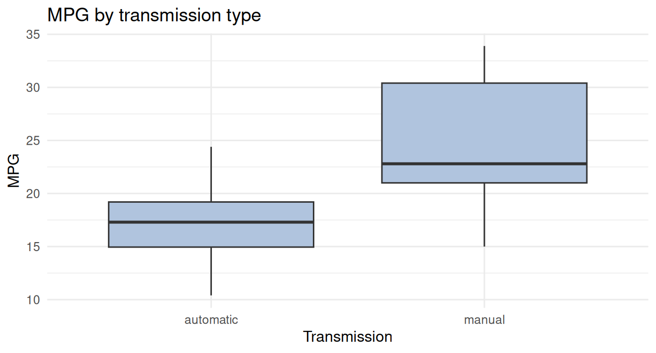

The boxplot suggests yes. Let’s quantify it:

t_result <- t.test(mpg ~ am, data = cars)
t_result

#> 
#>  Welch Two Sample t-test
#> 
#> data:  mpg by am
#> t = -3.8, df = 18, p-value = 0.001
#> alternative hypothesis: true difference in means between group 0 and group 1 is not equal to 0
#> 95 percent confidence interval:
#>  -11.28  -3.21
#> sample estimates:
#> mean in group 0 mean in group 1 
#>           17.15           24.39

How to read the output:

t = -3.77 — the test statistic. Bigger absolute value = stronger evidence the means differ.
df — degrees of freedom (Welch’s t-test uses fractional df, that’s fine).
p-value = 0.001374 — probability of seeing a difference this large (or larger) if the true means were actually equal. By the conventional cutoff of 0.05, this is “significant.”
95 percent confidence interval: -11.28, -3.21 — we’re 95% confident the true difference (automatic minus manual) is between about -11 and -3 MPG.
mean in group 0 = 17.15, mean in group 1 = 24.39 — the actual group means.

So manual cars in this dataset get around 7 MPG more than automatic cars on average, and the difference is statistically significant.

You can pull individual pieces out programmatically:

t_result$p.value

#> [1] 0.001374

t_result$conf.int

#> [1] -11.28  -3.21
#> attr(,"conf.level")
#> [1] 0.95

t_result$estimate

#> mean in group 0 mean in group 1 
#>           17.15           24.39

⚠️ “Significant” doesn’t mean “important”

A tiny effect with a huge sample will be “statistically significant.” A huge effect with a small sample may not be. Always look at the confidence interval and the effect size, not just the p-value.

Also: this comparison ignores that manuals tend to be in different cars than automatics (lighter, fewer cylinders, etc.). The honest answer to “does transmission cause better MPG” requires a model that controls for those things — that’s what regression is for.

Measuring association: correlation

Correlation measures how strongly two numeric variables move together, on a scale of -1 to 1.

cor(cars$wt, cars$mpg)

#> [1] -0.8677

A correlation of about -0.87: strong negative association. As weight goes up, MPG goes down.

cor.test() adds a hypothesis test (is the correlation different from zero?) and a confidence interval:

cor.test(cars$wt, cars$mpg)

#> 
#>  Pearson's product-moment correlation
#> 
#> data:  cars$wt and cars$mpg
#> t = -9.6, df = 30, p-value = 0.0000000001
#> alternative hypothesis: true correlation is not equal to 0
#> 95 percent confidence interval:
#>  -0.9338 -0.7441
#> sample estimates:
#>     cor 
#> -0.8677

For a whole correlation matrix:

cars |>
  select(mpg, hp, wt, drat, qsec) |>
  cor() |>
  round(2)

#>        mpg    hp    wt  drat  qsec
#> mpg   1.00 -0.78 -0.87  0.68  0.42
#> hp   -0.78  1.00  0.66 -0.45 -0.71
#> wt   -0.87  0.66  1.00 -0.71 -0.17
#> drat  0.68 -0.45 -0.71  1.00  0.09
#> qsec  0.42 -0.71 -0.17  0.09  1.00

Linear regression

Regression is the workhorse of applied statistics. The basic question: “How does the response variable change as the predictors change?”

A simple regression

Predict MPG from weight:

fit1 <- lm(mpg ~ wt, data = cars)
fit1

#> 
#> Call:
#> lm(formula = mpg ~ wt, data = cars)
#> 
#> Coefficients:
#> (Intercept)           wt  
#>       37.29        -5.34

The formula mpg ~ wt reads as “model mpg as a function of wt.” lm() returns a fitted model object — print it for a quick look, summary() for the full output:

summary(fit1)

#> 
#> Call:
#> lm(formula = mpg ~ wt, data = cars)
#> 
#> Residuals:
#>    Min     1Q Median     3Q    Max 
#> -4.543 -2.365 -0.125  1.410  6.873 
#> 
#> Coefficients:
#>             Estimate Std. Error t value             Pr(>|t|)    
#> (Intercept)   37.285      1.878   19.86 < 0.0000000000000002 ***
#> wt            -5.344      0.559   -9.56        0.00000000013 ***
#> ---
#> Signif. codes:  0 '***' 0.001 '**' 0.01 '*' 0.05 '.' 0.1 ' ' 1
#> 
#> Residual standard error: 3.05 on 30 degrees of freedom
#> Multiple R-squared:  0.753,  Adjusted R-squared:  0.745 
#> F-statistic: 91.4 on 1 and 30 DF,  p-value: 0.000000000129

What’s important here:

Coefficients: wt = -5.34 means each additional 1000 lbs of weight is associated with a 5.34-MPG decrease, on average.
Pr(>|t|) for wt: the p-value for “is this coefficient different from 0?” Tiny — yes.
R-squared = 0.75: 75% of the variation in MPG is explained by weight alone.
Residual standard error: typical prediction error in MPG units.

A multiple regression

Add more predictors with +:

fit2 <- lm(mpg ~ wt + hp + factor(cyl), data = cars)
summary(fit2)

#> 
#> Call:
#> lm(formula = mpg ~ wt + hp + factor(cyl), data = cars)
#> 
#> Residuals:
#>    Min     1Q Median     3Q    Max 
#> -4.261 -1.032 -0.321  0.928  5.395 
#> 
#> Coefficients:
#>              Estimate Std. Error t value            Pr(>|t|)    
#> (Intercept)   35.8460     2.0410   17.56 0.00000000000000027 ***
#> wt            -3.1814     0.7196   -4.42             0.00014 ***
#> hp            -0.0231     0.0120   -1.93             0.06361 .  
#> factor(cyl)6  -3.3590     1.4017   -2.40             0.02375 *  
#> factor(cyl)8  -3.1859     2.1705   -1.47             0.15370    
#> ---
#> Signif. codes:  0 '***' 0.001 '**' 0.01 '*' 0.05 '.' 0.1 ' ' 1
#> 
#> Residual standard error: 2.44 on 27 degrees of freedom
#> Multiple R-squared:  0.857,  Adjusted R-squared:  0.836 
#> F-statistic: 40.5 on 4 and 27 DF,  p-value: 0.0000000000487

Now we’re estimating the effect of weight after controlling for horsepower and cylinder count.

factor(cyl) tells R to treat cyl as a categorical variable rather than a number. The output gives you the difference between each level and a reference level (here, 4-cylinder).

Comparing models

anova() tests whether the bigger model is significantly better than the smaller one:

anova(fit1, fit2)

#> Analysis of Variance Table
#> 
#> Model 1: mpg ~ wt
#> Model 2: mpg ~ wt + hp + factor(cyl)
#>   Res.Df RSS Df Sum of Sq    F Pr(>F)   
#> 1     30 278                            
#> 2     27 161  3       118 6.58 0.0018 **
#> ---
#> Signif. codes:  0 '***' 0.001 '**' 0.01 '*' 0.05 '.' 0.1 ' ' 1

A small p-value means the extra predictors are pulling weight (so to speak).

AIC() and BIC() are alternative model-comparison metrics — lower is better:

AIC(fit1, fit2)

#>      df   AIC
#> fit1  3 166.0
#> fit2  6 154.5

Diagnostics

Before trusting a regression, look at the diagnostic plots. R’s built-in plot() on a model gives you four:

par(mfrow = c(2, 2))
plot(fit1)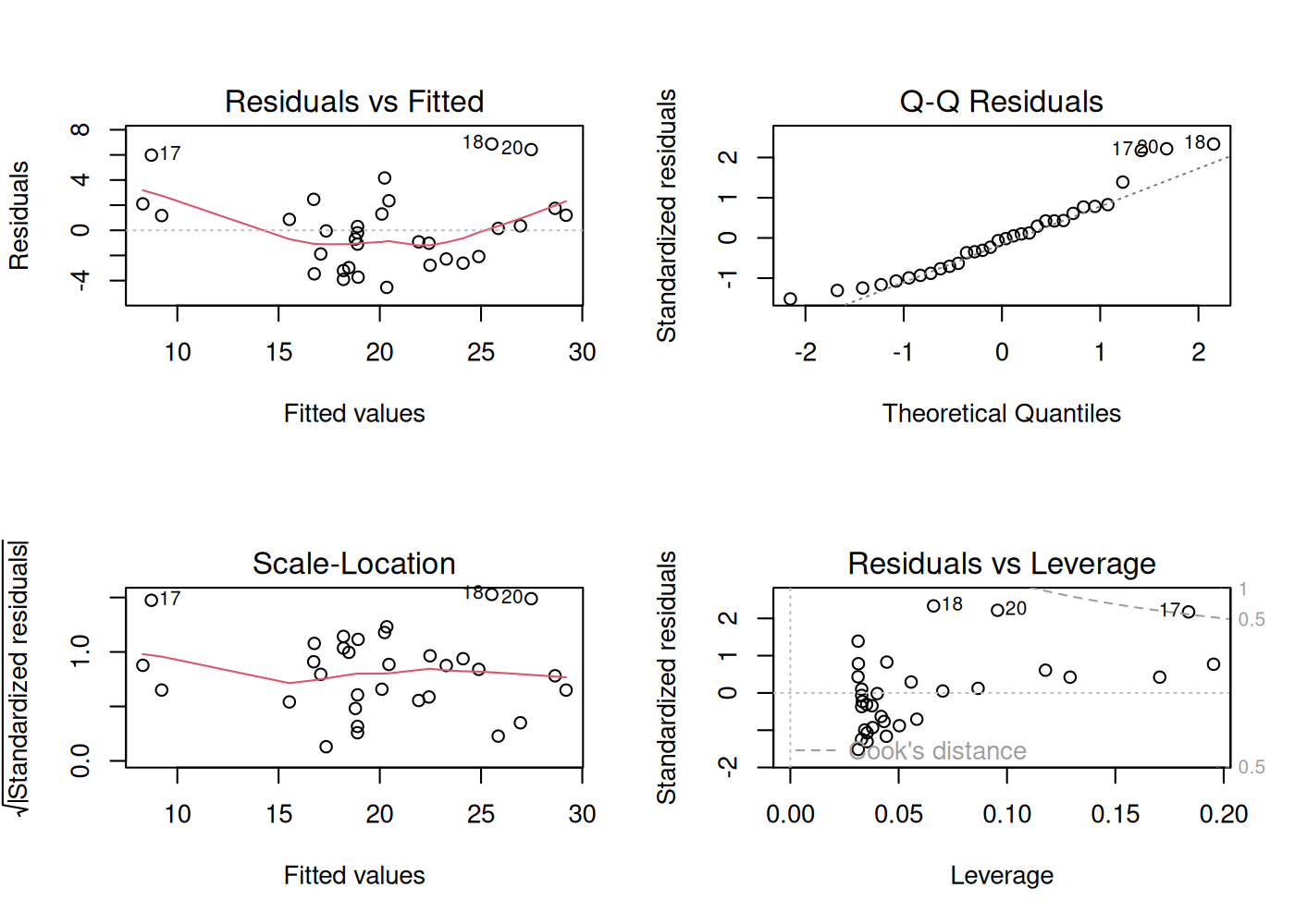

par(mfrow = c(1, 1))

What you’re looking for:

Residuals vs. Fitted — should look like a flat blob with no pattern. A curve suggests you’re missing nonlinearity.
Q-Q Residuals — should hug the diagonal line. Big departures = non-normal residuals.
Scale-Location — should be roughly flat. A trend means the variance changes with the fitted value (heteroscedasticity).
Residuals vs. Leverage — points with high Cook’s distance (top-right or bottom-right corners, past the dashed lines) are unusually influential. Investigate those rows.

Predictions

Once you have a model, you can predict new values:

new_cars <- tibble::tibble(wt = c(2.0, 3.5, 5.0))
predict(fit1, newdata = new_cars)

#>     1     2     3 
#> 26.60 18.58 10.56

Add a confidence interval for the mean response:

predict(fit1, newdata = new_cars, interval = "confidence")

#>     fit    lwr   upr
#> 1 26.60 24.824 28.37
#> 2 18.58 17.433 19.73
#> 3 10.56  8.249 12.88

Or a prediction interval for a single new observation (wider, because individual cars vary):

predict(fit1, newdata = new_cars, interval = "prediction")

#>     fit    lwr   upr
#> 1 26.60 20.128 33.06
#> 2 18.58 12.254 24.90
#> 3 10.56  3.926 17.20

Visualizing the fit

A simple regression line is one geom away in ggplot:

ggplot(cars, aes(x = wt, y = mpg)) +
  geom_point(size = 2.5, alpha = 0.8) +
  geom_smooth(method = "lm", se = TRUE, color = "steelblue") +
  labs(
    title = "MPG vs. Weight, with linear fit and 95% CI",
    x = "Weight (1000 lbs)", y = "MPG"
  ) +
  theme_minimal()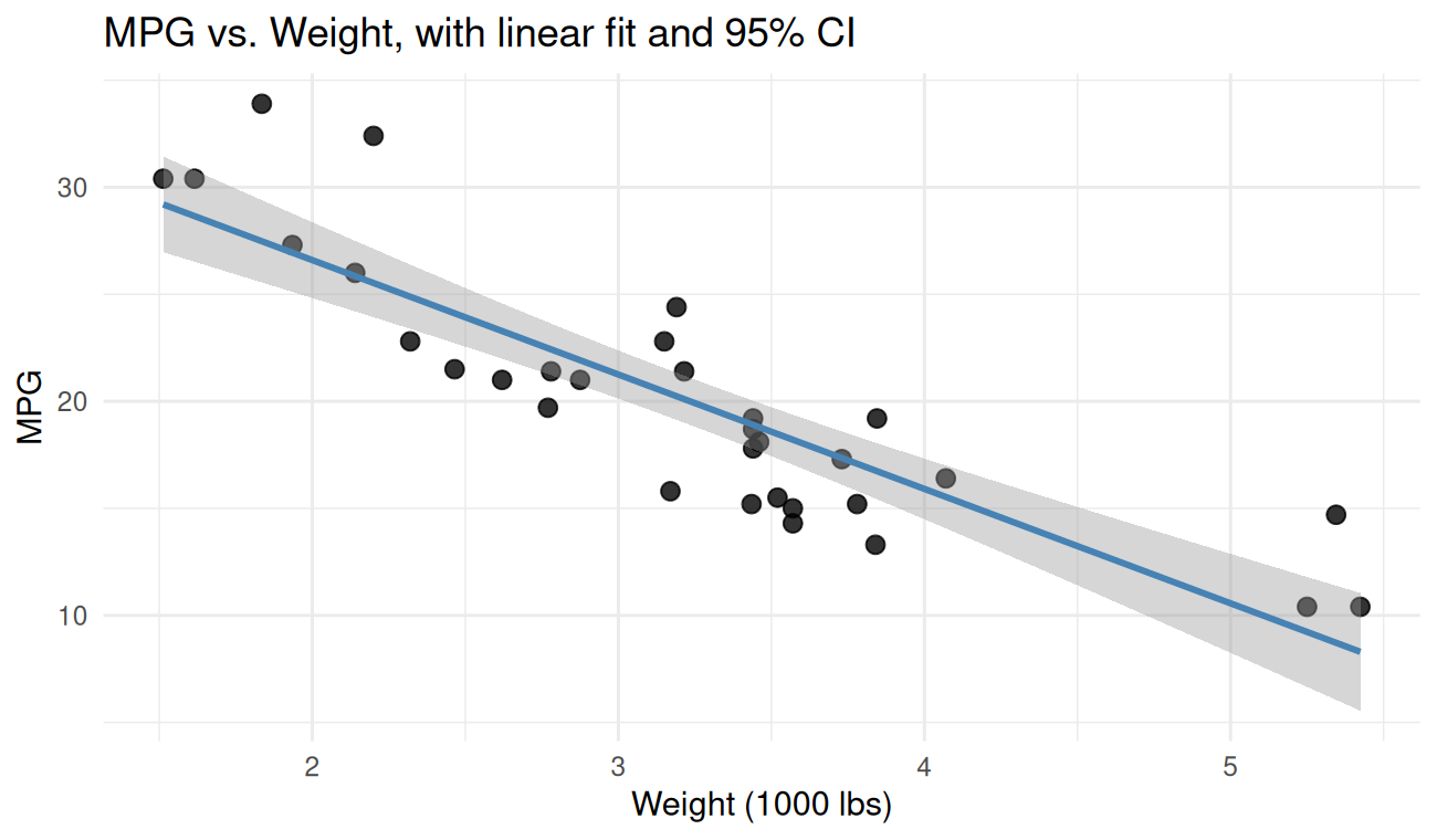

geom_smooth(method = "lm") is fitting the same model as lm(mpg ~ wt) under the hood and shading the confidence band.

A few other tests worth knowing

wilcox.test() — non-parametric alternative to the t-test (for non-normal data).
chisq.test() — chi-square test for independence between two categorical variables.
prop.test() — comparing proportions across groups.
aov() — ANOVA, for comparing means across more than two groups.
glm(..., family = binomial) — logistic regression, for binary outcomes.

The pattern is the same across all of them: a formula, a data argument, a summary or print of the result.

Putting it together

A complete mini-analysis: is MPG associated with weight, controlling for horsepower? Report the model, check assumptions, and predict MPG for a hypothetical new car.

fit <- lm(mpg ~ wt + hp, data = cars)
summary(fit)

#> 
#> Call:
#> lm(formula = mpg ~ wt + hp, data = cars)
#> 
#> Residuals:
#>    Min     1Q Median     3Q    Max 
#> -3.941 -1.600 -0.182  1.050  5.854 
#> 
#> Coefficients:
#>             Estimate Std. Error t value             Pr(>|t|)    
#> (Intercept) 37.22727    1.59879   23.28 < 0.0000000000000002 ***
#> wt          -3.87783    0.63273   -6.13            0.0000011 ***
#> hp          -0.03177    0.00903   -3.52               0.0015 ** 
#> ---
#> Signif. codes:  0 '***' 0.001 '**' 0.01 '*' 0.05 '.' 0.1 ' ' 1
#> 
#> Residual standard error: 2.59 on 29 degrees of freedom
#> Multiple R-squared:  0.827,  Adjusted R-squared:  0.815 
#> F-statistic: 69.2 on 2 and 29 DF,  p-value: 0.00000000000911

Coefficient interpretations: holding horsepower constant, each additional 1000 lbs of weight is associated with a -3.88-MPG decrease. Holding weight constant, each additional horsepower is associated with a -0.0318-MPG decrease.

Quick diagnostic look:

par(mfrow = c(1, 2))
plot(fit, which = c(1, 2))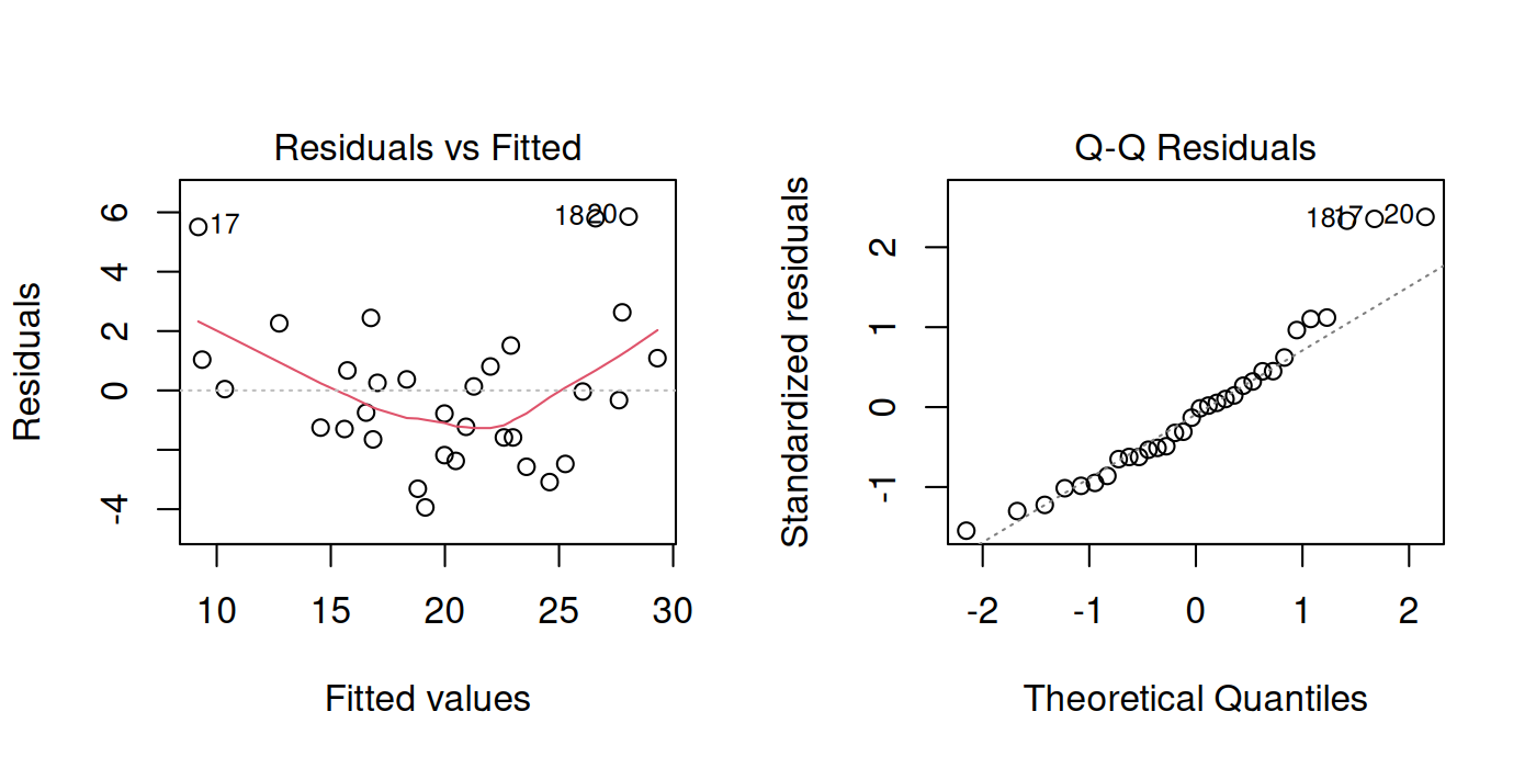

par(mfrow = c(1, 1))

Predict MPG for a 3500-lb car with 130 hp:

predict(fit, newdata = tibble::tibble(wt = 3.5, hp = 130), interval = "prediction")

#>     fit  lwr   upr
#> 1 19.52 14.1 24.95

That’s a complete (if minimal) regression analysis: fit, interpret, diagnose, predict.

✏️ Exercise 5.1 — Descriptive stats

Compute the mean, median, standard deviation, and IQR of cars$hp. Are the mean and median similar? What does that tell you about the distribution?

Show solution

mean(cars$hp)

#> [1] 146.7

median(cars$hp)

#> [1] 123

sd(cars$hp)

#> [1] 68.56

IQR(cars$hp)

#> [1] 83.5

The mean is noticeably higher than the median, which means the distribution is right-skewed — there are a few high-horsepower outliers pulling the mean up. A boxplot or histogram would confirm.

ggplot(cars, aes(x = hp)) +
  geom_histogram(bins = 12, fill = "steelblue", color = "white") +
  theme_minimal()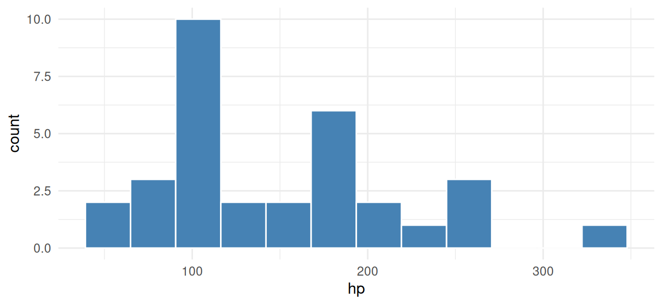

✏️ Exercise 5.2 — A t-test

Test whether 4-cylinder cars have a different mean MPG than 8-cylinder cars. Report the p-value, the 95% CI, and a one-sentence interpretation.

Show solution

sub <- cars |> filter(cyl %in% c(4, 8))
t.test(mpg ~ cyl, data = sub)

#> 
#>  Welch Two Sample t-test
#> 
#> data:  mpg by cyl
#> t = 7.6, df = 15, p-value = 0.000002
#> alternative hypothesis: true difference in means between group 4 and group 8 is not equal to 0
#> 95 percent confidence interval:
#>   8.319 14.809
#> sample estimates:
#> mean in group 4 mean in group 8 
#>           26.66           15.10

The mean MPG of 4-cylinder cars is roughly 11 MPG higher than 8-cylinder cars (95% CI ~9 to 13), and the p-value is tiny — the difference is far more than chance.

✏️ Exercise 5.3 — A regression

Fit a model that predicts MPG from weight, horsepower, and cylinder count (treat cyl as a factor). Which coefficients are statistically significant? What’s the R-squared?

Show solution

fit <- lm(mpg ~ wt + hp + factor(cyl), data = cars)
summary(fit)

#> 
#> Call:
#> lm(formula = mpg ~ wt + hp + factor(cyl), data = cars)
#> 
#> Residuals:
#>    Min     1Q Median     3Q    Max 
#> -4.261 -1.032 -0.321  0.928  5.395 
#> 
#> Coefficients:
#>              Estimate Std. Error t value            Pr(>|t|)    
#> (Intercept)   35.8460     2.0410   17.56 0.00000000000000027 ***
#> wt            -3.1814     0.7196   -4.42             0.00014 ***
#> hp            -0.0231     0.0120   -1.93             0.06361 .  
#> factor(cyl)6  -3.3590     1.4017   -2.40             0.02375 *  
#> factor(cyl)8  -3.1859     2.1705   -1.47             0.15370    
#> ---
#> Signif. codes:  0 '***' 0.001 '**' 0.01 '*' 0.05 '.' 0.1 ' ' 1
#> 
#> Residual standard error: 2.44 on 27 degrees of freedom
#> Multiple R-squared:  0.857,  Adjusted R-squared:  0.836 
#> F-statistic: 40.5 on 4 and 27 DF,  p-value: 0.0000000000487

wt has a clearly significant negative coefficient. hp and the cylinder-count contrasts get smaller and may no longer be significant once weight is in the model — they’re correlated with weight (heavier cars tend to have more cylinders and more horsepower), so a lot of the “effect” of cylinders is really just weight. Adjusted R-squared should be around 0.83.

What’s next

You can now load data, manipulate it, plot it, and run real statistical analyses on it. The last two lessons stop adding new tools and start showing how to package up an analysis so someone else (or future-you) can run it again. Lesson 6 is R Markdown — the document format this whole course is written in.

← Previous Lesson 4: Data Visualization Next → Lesson 6: Reproducible Reports

Lesson 5: Statistics with R

Cavan Donohoe

Statistics with R

Setup

Descriptive statistics

Comparing two groups: the t-test

Measuring association: correlation

Linear regression

A simple regression

A multiple regression

Comparing models

Diagnostics

Predictions

Visualizing the fit

A few other tests worth knowing

Putting it together

What’s next